《动手学深度学习（PyTorch版）》第2章 预备知识 读书笔记

目录

• 2.1 数据操作
• 2.2 数据预处理
• 2.3 线性代数
• 2.4 微积分
• 2.5 自动微分
• 2.6 概率
• 2.7 查阅文档
• 本章核心总结（必看）
• 结语

---

  这一章是全书的"工具箱"——我们要把后面写代码需要的基础操作全部过一遍。别嫌基础，80%的深度学习bug都出在这些基础操作上（张量维度不对、索引越界、梯度没清零……），所以这一章一定要动手敲代码。

  这一章的内容包括：PyTorch张量操作、数据预处理、线性代数、微积分、自动微分、概率统计。每一部分我们都配了可运行的代码和真实输出。

2.1 数据操作

  在深度学习中，所有数据都以**张量（tensor）**的形式存储和运算。你可以把张量理解为多维数组：0维是标量，1维是向量，2维是矩阵，3维及以上就是张量。

2.1.1 入门

import torch

# 创建张量
x = torch.arange(12, dtype=torch.float32)
print("x =", x)
print("x.shape =", x.shape)   # 形状
print("x.numel() =", x.numel())  # 元素总数

# 改变形状（不改变元素数量和值）
X = x.reshape(3, 4)
print("X = x.reshape(3,4):\n", X)

# 创建特殊张量
print("torch.zeros((2,3,4)):\n", torch.zeros((2, 3, 4)))
print("torch.ones((2,3,4)) shape:", torch.ones((2, 3, 4)).shape)
print("torch.randn(3,4):\n", torch.randn(3, 4))

运行结果：

x = tensor([ 0.,  1.,  2.,  3.,  4.,  5.,  6.,  7.,  8.,  9., 10., 11.])
x.shape = torch.Size([12])
x.numel() = 12
X = x.reshape(3,4):
 tensor([[ 0.,  1.,  2.,  3.],
        [ 4.,  5.,  6.,  7.],
        [ 8.,  9., 10., 11.]])

  要点：reshape 只改变张量的"视图"，不改变底层数据。numel() 返回元素总数，shape 返回各维度大小。

2.1.2 运算符

x = torch.tensor([1.0, 2, 4, 8])
y = torch.tensor([2, 2, 2, 2])
print("x + y:", x + y)
print("x * y:", x * y)
print("x ** y:", x ** y)
print("torch.exp(x):", torch.exp(x))

# 张量拼接
X = torch.arange(12, dtype=torch.float32).reshape((3, 4))
Y = torch.tensor([[2.0, 1, 4, 3], [1, 2, 3, 4], [4, 3, 2, 1]])
print("cat dim=0:\n", torch.cat((X, Y), dim=0))  # 按行拼接
print("cat dim=1:\n", torch.cat((X, Y), dim=1))  # 按列拼接
print("X == Y:\n", X == Y)
print("X.sum():", X.sum())

运行结果：

x + y: tensor([ 3.,  4.,  6., 10.])
x * y: tensor([ 2.,  4.,  8., 16.])
x ** y: tensor([ 1.,  4., 16., 64.])
torch.exp(x): tensor([2.7183e+00, 7.3891e+00, 5.4598e+01, 2.9810e+03])
X.sum(): tensor(66.)

2.1.3 广播机制

  当两个张量形状不同时，PyTorch会尝试广播（broadcasting）——把小的张量"复制扩展"到和大的张量一样的形状，再进行运算。

a = torch.arange(3).reshape((3, 1))  # 3行1列
b = torch.arange(2).reshape((1, 2))  # 1行2列
print("a + b (broadcast to 3x2):\n", a + b)

运行结果：

a + b (broadcast to 3x2):
 tensor([[0, 1],
        [1, 2],
        [2, 3]])

  a（3×1）被广播成3×2（每列复制），b（1×2）被广播成3×2（每行复制），然后逐元素相加。

2.1.4 索引和切片

print("X[-1]:", X[-1])       # 最后一行
print("X[1:3]:\n", X[1:3])   # 第2、3行
X[1, 2] = 9                   # 修改单个元素
X[0:2, :] = 12                # 修改区域

2.1.5 节省内存

  Y = Y + X 会新分配内存给Y，而 Y += X 或 Y[:] = Y + X 是原地操作，不分配新内存。训练模型时参数更新要用原地操作，否则内存会爆。

before = id(Y)
Y = Y + X
print("id(Y) changed:", id(Y) != before)  # True，新分配了内存

Z = torch.zeros_like(Y)
Z[:] = X + Y  # 原地操作，不分配新内存

运行结果：

id(Y) changed after Y = Y + X: True
id(Z) before: 4484860864
id(Z) after Z[:] = X+Y: 4484860864
id(X) unchanged after X += Y: True

2.1.6 转换为其他Python对象

A = X.numpy()           # 张量 → numpy数组
B = torch.from_numpy(A) # numpy数组 → 张量
a = torch.tensor([3.5])
print("a.item():", a.item())  # 标量张量 → Python标量

2.2 数据预处理

  真实世界的数据不是干净的张量，而是CSV、JSON、数据库里的"脏数据"。我们需要用pandas读取、清洗，再转成张量。

2.2.1 读取数据集

import os
import pandas as pd

# 创建一个小数据集
os.makedirs(os.path.join('..', 'data'), exist_ok=True)
data_file = os.path.join('..', 'data', 'house_tiny.csv')
with open(data_file, 'w') as f:
    f.write('NumRooms,Alley,Price\n')
    f.write('NA,Pave,127500\n')
    f.write('2,NA,106000\n')
    f.write('4,NA,178100\n')
    f.write('NA,NA,140000\n')

data = pd.read_csv(data_file)
print(data)

运行结果：

   NumRooms Alley   Price
0       NaN  Pave  127500
1       2.0   NaN  106000
2       4.0   NaN  178100
3       NaN   NaN  140000

2.2.2 处理缺失值

  处理缺失值（NaN）的常用方法：插值（用均值/中位数填充数值型缺失）和删除。对于类别型缺失，用 get_dummies 转成one-hot编码。

inputs, outputs = data.iloc[:, 0:2], data.iloc[:, 2]
inputs = inputs.fillna(inputs.mean(numeric_only=True))  # 数值列用均值填充
print("After fillna:\n", inputs)
inputs = pd.get_dummies(inputs, dummy_na=True)  # 类别列转one-hot
print("After get_dummies:\n", inputs)

运行结果：

After fillna:
    NumRooms Alley
0       3.0  Pave
1       2.0   NaN
2       4.0   NaN
3       3.0   NaN
After get_dummies:
    NumRooms  Alley_Pave  Alley_nan
0       3.0        True      False
1       2.0       False       True
2       4.0       False       True
3       3.0       False       True

2.2.3 转换为张量格式

import numpy as np
X = torch.tensor(inputs.to_numpy(dtype=np.float32))
y = torch.tensor(outputs.to_numpy(dtype=np.float32))
print("X tensor:\n", X)
print("y tensor:", y)

运行结果：

X tensor:
 tensor([[3., 1., 0.],
        [2., 0., 1.],
        [4., 0., 1.],
        [3., 0., 1.]])
y tensor: tensor([127500., 106000., 178100., 140000.])

2.3 线性代数

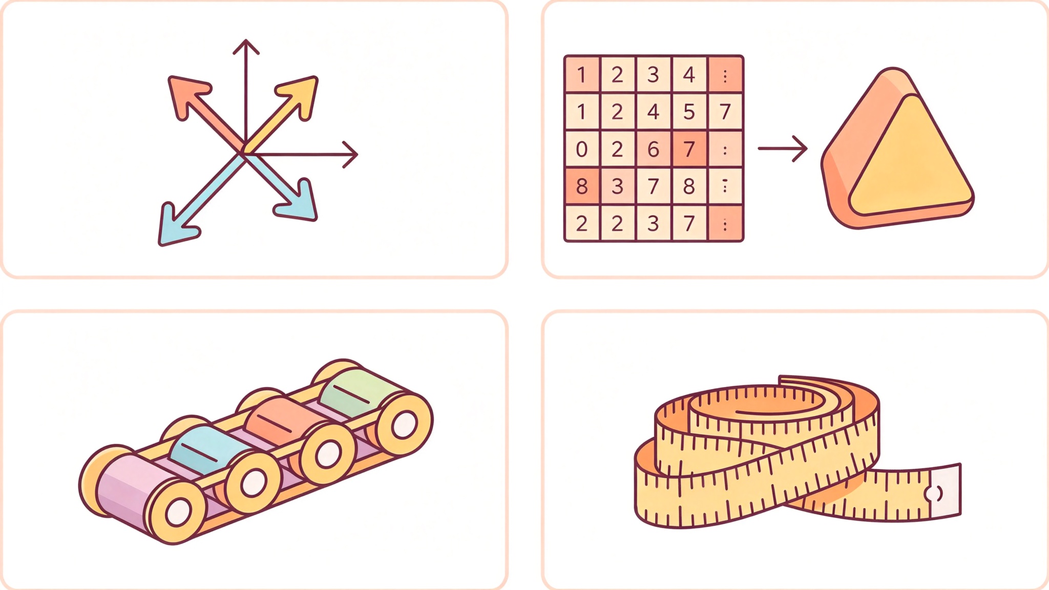
  线性代数是深度学习的数学基础。神经网络的每一层本质上都是矩阵乘法。我们快速过一遍核心概念。

2.3.1-2.3.4 标量、向量、矩阵、张量

# 标量
x = torch.tensor(3.0)
# 向量
v = torch.arange(4, dtype=torch.float32)
# 矩阵
A = torch.arange(20, dtype=torch.float32).reshape(5, 4)
print("A.T (转置):\n", A.T)
# 张量
T = torch.arange(24, dtype=torch.float32).reshape(2, 3, 4)

2.3.5 张量算法的基本性质

  两个同形状张量的逐元素运算（Hadamard积）：A * B。标量和张量的运算会广播到每个元素。

2.3.6 降维

print("A.sum():", A.sum())           # 所有元素求和
print("A.sum(axis=0):", A.sum(axis=0))  # 按行求和（消去行维度）
print("A.mean():", A.mean())         # 平均值
print("A.cumsum(axis=0):\n", A.cumsum(axis=0))  # 累加求和

运行结果：

A.sum(): tensor(190.)
A.sum(axis=0): tensor([40., 45., 50., 55.])
A.mean(): tensor(9.5000)

2.3.7 点积

x = torch.arange(4, dtype=torch.float32)
y = torch.ones(4, dtype=torch.float32)
print("torch.dot(x, y):", torch.dot(x, y))  # 0*1 + 1*1 + 2*1 + 3*1 = 6

2.3.8-2.3.9 矩阵-向量积、矩阵-矩阵乘法

A = torch.arange(20, dtype=torch.float32).reshape(5, 4)
x = torch.arange(4, dtype=torch.float32)
print("torch.mv(A, x):", torch.mv(A, x))  # 矩阵×向量

B = torch.ones(4, 3)
print("torch.mm(A, B) shape:", torch.mm(A, B).shape)  # 矩阵×矩阵

运行结果：

torch.mv(A, x): tensor([ 14.,  38.,  62.,  86., 110.])
torch.mm(A, B) shape: torch.Size([5, 3])

2.3.10 范数

  范数（norm）衡量向量/矩阵的"大小"。

• L2范数（欧几里得距离）：||x||₂ = √(Σxᵢ²)
• L1范数：||x||₁ = Σ|xᵢ|
• Frobenius范数：矩阵的L2范数

u = torch.tensor([3.0, -4.0])
print("L2 norm:", torch.norm(u))          # 5.0
print("L1 norm:", torch.abs(u).sum())     # 7.0
v = torch.ones((4, 9))
print("Frobenius norm:", torch.norm(v))    # 6.0

运行结果：

L2 norm: tensor(5.)
L1 norm: tensor(7.)
Frobenius norm: tensor(6.)

2.4 微积分

  微积分是优化算法的基础。训练神经网络本质上就是求损失函数的最小值，而求最小值需要导数和梯度。

2.4.1 导数和微分

  导数 f'(x) 衡量函数在某点的变化率，几何上是切线的斜率。

$$f^{\prime }(x)=\underset{h\to 0}{\lim }\frac{f(x+h)-f(x)}{h}$$

2.4.2 偏导数

  多元函数对某个变量求导，其他变量视为常数，就是偏导数 ∂f/∂xᵢ。

2.4.3 梯度

  梯度（gradient）是所有偏导数组成的向量，指向函数增长最快的方向。优化时我们沿梯度反方向更新参数。

$$\nabla f(\mathbf{x})={\left[\frac{\partial f}{\partial x_1},\frac{\partial f}{\partial x_2},\dots ,\frac{\partial f}{\partial x_n}\right]}^T$$

2.4.4 链式法则

  复合函数求导用链式法则：dy/dx = (dy/du) × (du/dx)。这是反向传播算法的数学基础。

2.5 自动微分

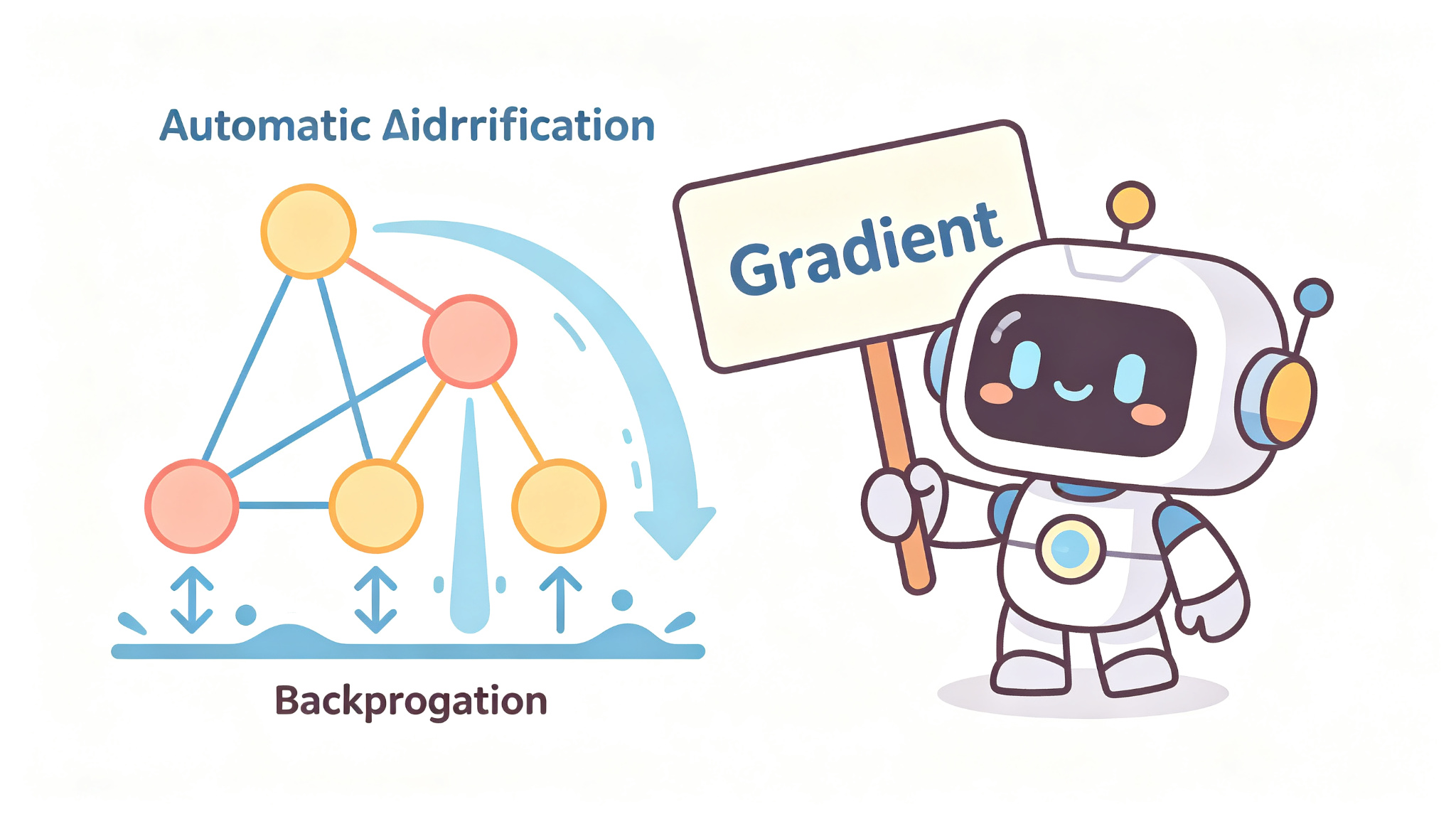
  深度学习模型可能有几十亿个参数，手动求导不现实。PyTorch的自动微分（autograd） 能自动计算梯度——你只需要写前向传播，反向传播自动搞定。

2.5.1 一个简单的例子

  假设 y = 2x·x，我们想求 dy/dx。手动算：dy/dx = 4x。

x = torch.arange(4.0)
x.requires_grad_(True)  # 告诉PyTorch需要跟踪x的梯度
y = 2 * torch.dot(x, x)  # y = 2*(0²+1²+2²+3²) = 28
y.backward()  # 反向传播，计算梯度
print("x.grad:", x.grad)  # 应该等于 4x = [0, 4, 8, 12]
print("x.grad == 4*x:", x.grad == 4 * x)

运行结果：

x.grad (dy/dx = 4x): tensor([ 0.,  4.,  8., 12.])
x.grad == 4*x: tensor([True, True, True, True])

  注意：梯度是累积的，每次反向传播前要 x.grad.zero_() 清零，否则会叠加。

2.5.2 非标量变量的反向传播

  当y不是标量时，y.backward() 会报错。需要先求和：y.sum().backward()。

x.grad.zero_()
y = x * x
y.sum().backward()
print("x.grad:", x.grad)  # [0, 2, 4, 6]

2.5.3 分离计算

  有时我们想把某些计算"冻结"，不让梯度传过去。用 detach()：

x.grad.zero_()
y = x * x
u = y.detach()  # u被当作常数，梯度不会传到y
z = u * x
z.sum().backward()
print("x.grad == u:", x.grad == u)  # True，dz/dx = u

2.5.4 Python控制流的梯度计算

  自动微分甚至能处理包含Python控制流（if/while）的函数：

def f(a):
    b = a * 2
    while b.norm() < 1000:
        b = b * 2
    if b.sum() > 0:
        c = b
    else:
        c = 100 * b
    return c

a = torch.randn(size=(), requires_grad=True)
d = f(a)
d.backward()
print("a.grad == d/a:", a.grad == d / a)  # True

运行结果：

a = tensor(1.3310, requires_grad=True)
f(a) = tensor(1362.9602)
a.grad = tensor(1024.)
a.grad == d/a: tensor(True)

2.6 概率

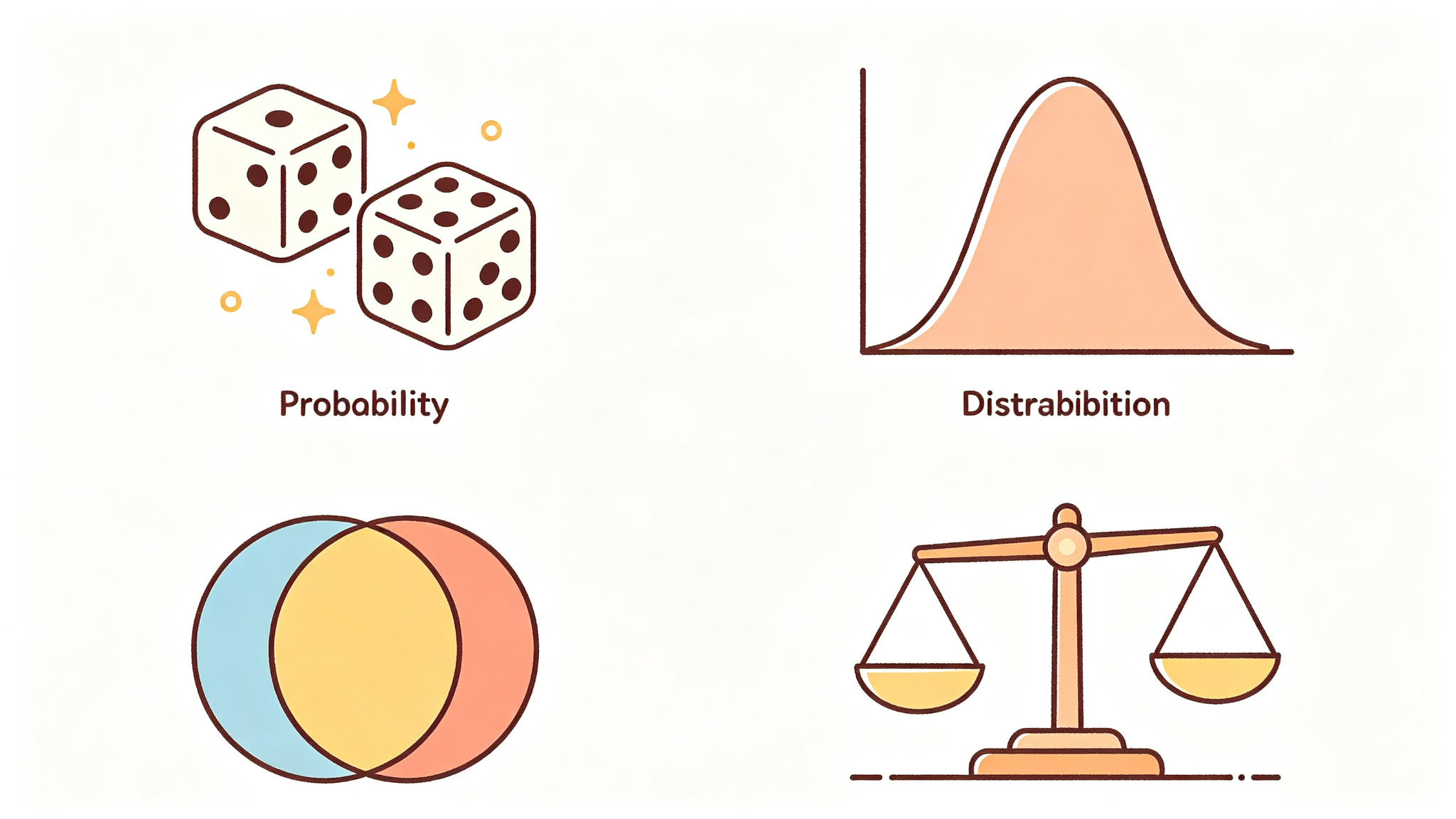
  深度学习和概率统计密不可分：模型的预测本质上是概率分布，损失函数常来自最大似然估计，正则化对应贝叶斯先验。

2.6.1 基本概率论

  我们用掷骰子来理解概率。理论上每个面的概率是1/6 ≈ 0.1667。模拟1000次掷骰子：

fair_probs = torch.ones([6]) / 6
counts = torch.multinomial(fair_probs, 1000, replacement=True)
roll_counts = torch.bincount(counts, minlength=6)
print("Counts:", roll_counts)
print("Empirical probs:", roll_counts.float() / 1000)

运行结果：

Counts for 1000 rolls: tensor([185, 177, 167, 180, 128, 163])
Empirical probabilities: tensor([0.1850, 0.1770, 0.1670, 0.1800, 0.1280, 0.1630])

  大数定律：试验次数越多，经验概率越接近理论概率。

n=     1: P(6)=1.0000, P(1)=0.0000
n=    10: P(6)=0.2000, P(1)=0.2000
n=   100: P(6)=0.2100, P(1)=0.1600
n=  1000: P(6)=0.1720, P(1)=0.1570
n= 10000: P(6)=0.1614, P(1)=0.1732

2.6.2 处理多个随机变量

  联合概率 P(A,B)：两个事件同时发生的概率。条件概率 P(A|B)：在B发生的条件下A发生的概率。

# 掷两个骰子，P(和为7)
rolls1 = torch.multinomial(fair_probs, 10000, replacement=True)
rolls2 = torch.multinomial(fair_probs, 10000, replacement=True)
sum7 = (rolls1 + rolls2 == 5).float().mean()
print(f"P(sum=7): {sum7:.4f} (theoretical: 0.1667)")

运行结果：

P(sum of two dice = 7): 0.1585 (theoretical: 0.1667)

2.6.3 期望和方差

  期望 E[X]：随机变量的平均值。方差 Var(X)：随机变量偏离期望的程度。

dice_values = torch.arange(1, 7, dtype=torch.float32)
expected = (dice_values * fair_probs).sum()
variance = ((dice_values - expected) ** 2 * fair_probs).sum()
print(f"E[X] = {expected:.4f} (theoretical: 3.5)")
print(f"Var(X) = {variance:.4f} (theoretical: 2.9167)")

# 正态分布采样验证
samples = torch.randn(10000)
print(f"Mean: {samples.mean():.4f}, Std: {samples.std():.4f}")

运行结果：

E[X] (dice) = 3.5000 (theoretical: 3.5)
Var(X) (dice) = 2.9167 (theoretical: 2.9167)
Std(X) = 1.7078
Mean of 10000 standard normal samples: -0.0096 (theoretical: 0)
Std of 10000 standard normal samples: 0.9949 (theoretical: 1)

2.7 查阅文档

  PyTorch有几百个函数，记不住很正常。学会查文档是必备技能。

# 查找模块中的所有函数和类
print(dir(torch.distributions)[:10])

# 查找特定函数的用法
help(torch.ones)
# 或在Jupyter中用 ?torch.ones

运行结果：

torch.distributions modules (first 10):
['AbsTransform', 'AffineTransform', 'Bernoulli', 'Beta', 'Binomial', ...]

ones(*size, *, out=None, dtype=None, ...) -> Tensor
Returns a tensor filled with the scalar value `1`...

本章核心总结（必看）

  一句话概括：第2章搭建了深度学习的"工具箱"——张量是数据载体，线性代数是运算语言，微积分和自动微分是优化基础，概率统计是建模思维。

  核心概念清单：

• 张量操作：创建(arange/zeros/ones/randn)、变形(reshape)、运算(逐元素/cat/sum)、广播机制、索引切片、原地操作(+=/[:])
• 数据预处理：pandas读取CSV → 缺失值填充(均值) → 类别变量one-hot(get_dummies) → 转张量
• 线性代数：标量/向量/矩阵/张量、转置、降维(sum/mean)、点积(dot)、矩阵乘法(mm/mv)、范数(norm)
• 微积分：导数→偏导数→梯度→链式法则，梯度下降沿梯度反方向更新
• 自动微分：requires_grad_(True) 开启跟踪 → 前向计算 → backward() 反向传播 → .grad 取梯度，记得 zero_() 清零
• 概率：大数定律、联合/条件概率、期望E[X]、方差Var(X)、正态分布

结语

  第2章的预备知识就到这里。这一章内容多但都是基础，建议大家把代码亲手跑一遍——看懂和会用之间隔着100次报错。

  下一章我们将进入线性神经网络，开始真正的机器学习之旅：线性回归、softmax回归、图像分类。我们会用这一章学的张量操作和自动微分，从零实现第一个神经网络！

转载自 CSDN-专业IT技术社区

原文链接：https://blog.csdn.net/2302_80961196/article/details/165117704